Pete Lawrence is your guide to viewing variable stars so you can record their changes in brightness
Although it may not be obvious at first sight, many stars vary in brightness over time. Some of these variable stars change magnitude on predictable timescales, others are less regular. Recording the variations is a rewarding and straightforward form of observing which ultimately helps decode how certain stars work. In this article we’ll look at different types of variable, how to observe them and how to interpret the results. We’ll also give you some examples to get you started.
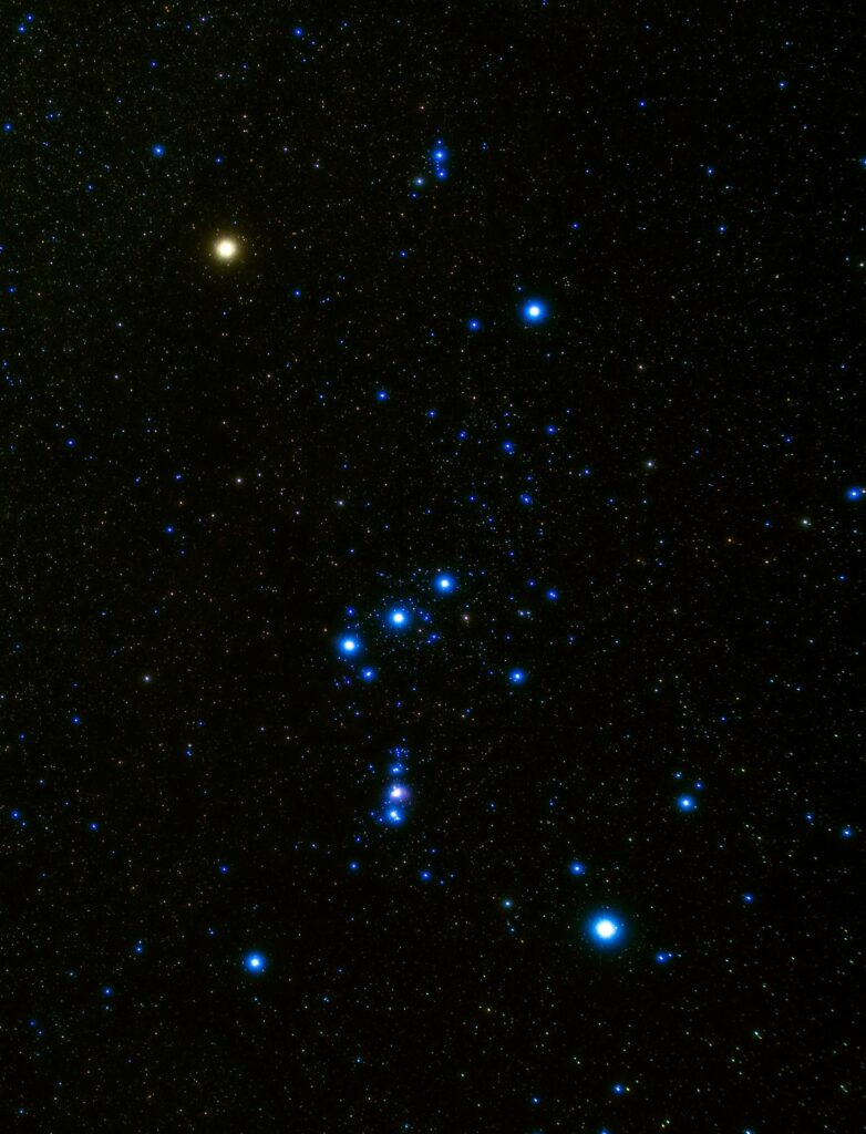
A star’s brightness is quantified by its magnitude. Some stars remain at constant magnitude, some vary a little and some vary a lot. Indeed, some stars become bright enough to change the visual appearance of their host constellation, such as Betelgeuse (Alpha (α) Orionis) and Mira (Omicron (ο) Ceti) (see ‘Six variable stars to get you started’ below). Variability can occur on a predictable basis or can be highly irregular. The majority of variable stars appear to vary indefinitely, but some vary just once, with extreme examples being supernovae.
Variation in magnitude is either caused by external factors or by internal changes within the star; those in the first group are known as extrinsic variables, while those in the second are called intrinsic variables. An eclipsing binary such as Algol (Beta (β) Persei) is an example of an extrinsic variable; its observed brightness variation is due to a dimmer star passing in front of a brighter one with a very predictable period.
Many intrinsic variables pulse as a result of changes in the opacity of the star’s outer layers. When the star is at minimum size, the outer layers are opaque and resistant to the passage of radiation from the star’s fusion core. Consequently, the outer layers swell and as they do so their opacity drops and energy escapes more easily. The outer layers subsequently shrink back towards the core and the cycle repeats. Variations in the temperature of the outer layers, and their size, affect the star’s luminosity.
Getting started
Stars with predictable variation are great to observe when starting out because they give you something to compare your results against. Don’t research where the star should be in its cycle before you begin, though: observe it and determine the extremes yourself first. It’ll give a great confidence boost when you discover you’re in sync with other observations.
Less predictable, irregular variables take the subject to a new level and here you could be making cutting-edge observations of your own. Has the star done something odd? Is it brighter or dimmer than it should be? Based on the skill set derived from observing regular variables, you could be the first person to record something exciting.
Once you’ve built your variable star observing toolbox, you’re set for the really unpredictable stuff such as eruptive variables, cataclysmic variables, flare stars, classical novae and ultimately supernovae. The last ‘local’ supernova occurred in the Large Magellanic Cloud, a dwarf satellite galaxy of the Milky Way, in 1987. Who knows when the next one will occur, but at least you’ll be ready for it. There are many categories of variable star as we’ve shown below.
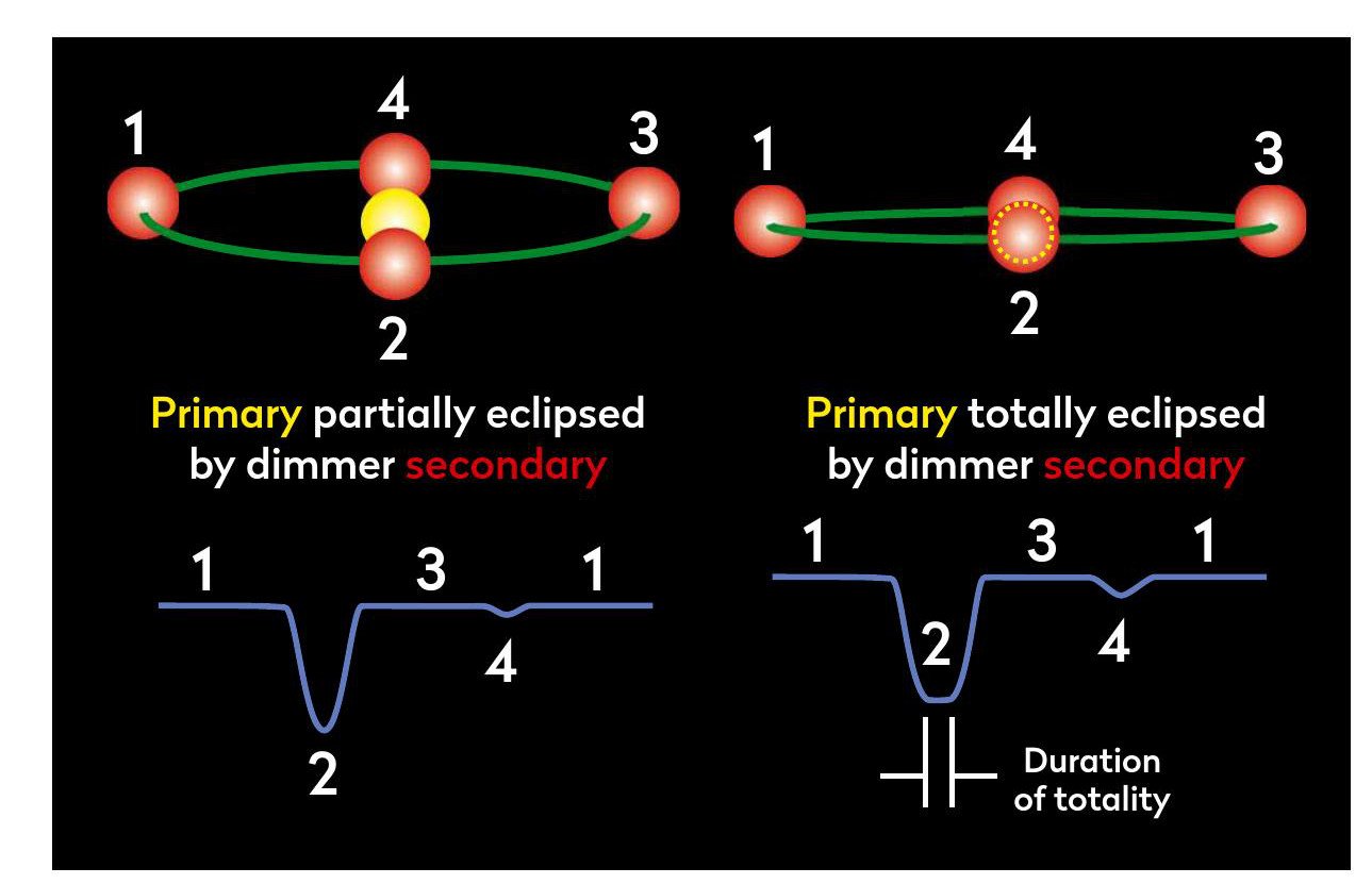
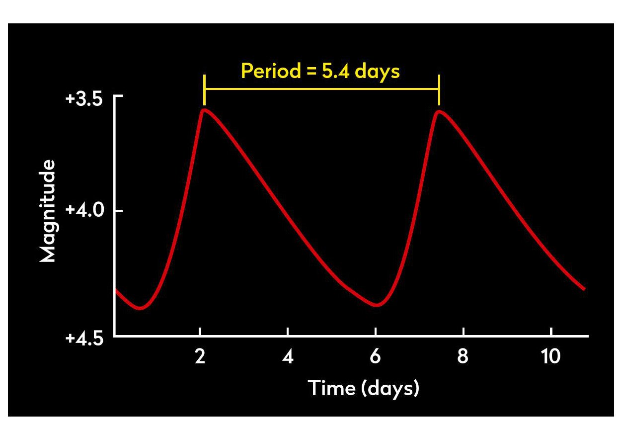
The ultimate goal of variable star observing is to plot a star’s light curve. There is nothing complex about this, it’s basically a graph with time along the horizontal axis and magnitude along the vertical axis, but it can show a great deal about the variable. For example, create a detailed light curve for an eclipsing binary and the curve’s shape will tell whether you are seeing a partial or full eclipse of the primary star. A partial eclipse shows a constantly changing curve, while a total shows a curve which ‘bottoms out’ at minimum brightness.
The longest period eclipsing binary is Almaaz (Epsilon (ε) Aurigae), with a period of 27 years. An eclipse dims the system from mag. +2.9 to +3.8, bottoming out for a couple of years, indicating a total eclipse of the primary. However, the brightness increases slightly mid-eclipse, before falling back to minimum again. One suggestion for this odd behaviour is that the secondary is a B-type star embedded in a thick obscuring disc of material aligned nearly edge-on to us. The minor peak occurs when the disc’s central hole allows some of the primary’s light through.
Types of variable star
Here’s what’s happening to cause changes in brightness in the most common variables
INTRINSIC VARIABLES
Variability caused by internal factors
Eruptive variables
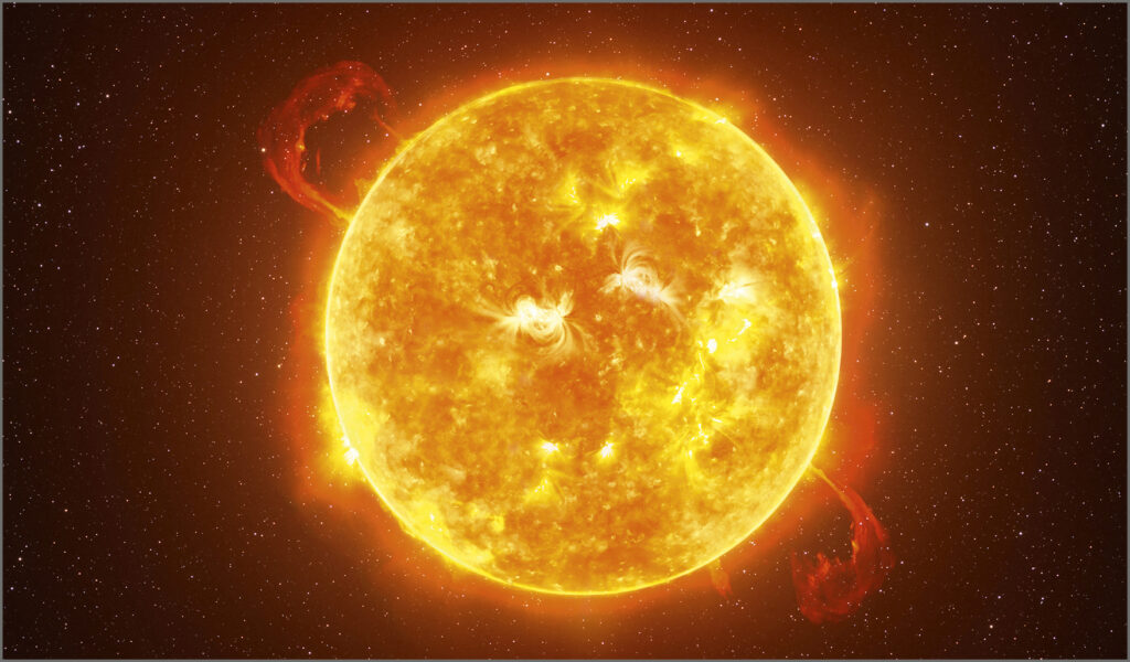
Output varies due to violent processes and flares within the star’s surface and atmospheric layers. Examples include:
Gamma Cassiopeiae
FU Orionis
RS Canum Venaticorum
S Doradus
R Coronae Borealis and UV Ceti
These include irregular variables and rapid irregulars. Some eruptives eject material into the surrounding space to interact with the interstellar medium. Eruptive Wolf–Rayet stars also come under this class: massive, highly evolved stars that continually eject gas into space.
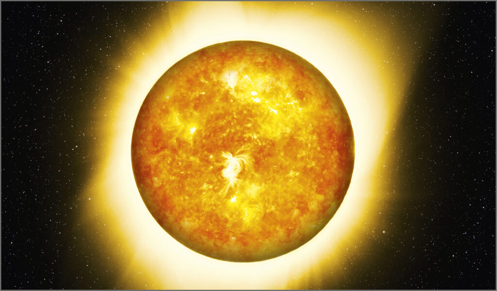
Pulsating variables
Stars which grow and shrink their outer layers, often in periodic fashion. The processes are linked to the star’s internal energy generation, swelling when heating up then shrinking when cooling, the cycle then repeating. Pulsation may be symmetrical (radial) or asymmetrical (non-radial).
Examples include:
Delta Cephei, the prototype of all Cepheid-type variable stars
RR Lyrae ZZ Ceti Mira, the prototype of Mira-type variable stars
Betelgeuse, a semi-regular pulsating variable.
Cataclysmic variables
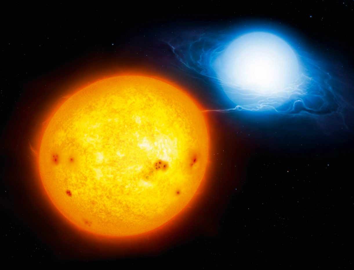
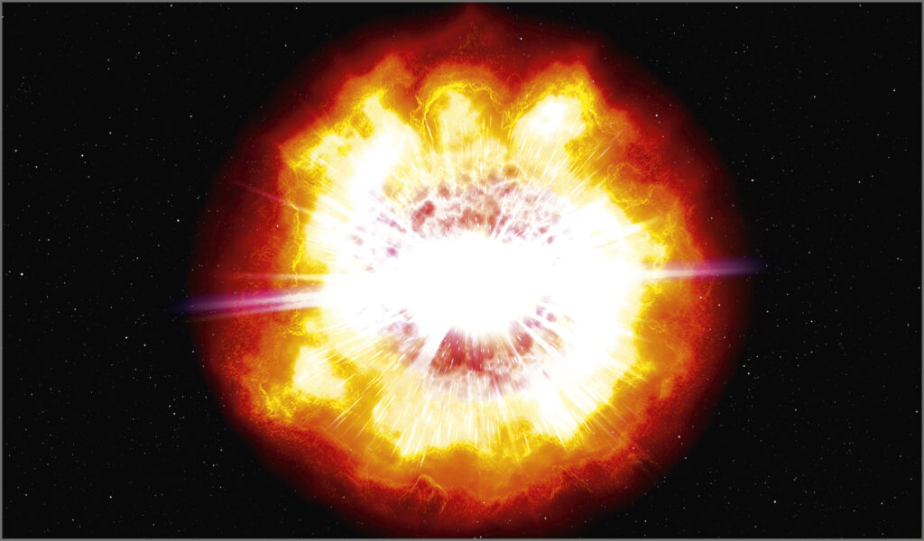
Thermonuclear outbursts in a star’s surface layers produce a nova or, when deep within a star’s interior, a supernova. Novae are typically close binaries: a white dwarf with a giant, subgiant or dwarf companion. U Geminorum and SS Cygni are examples of dwarf novae.
Supernovae show outburst brightening of 20 magnitudes or more, followed by a slow fade. This results in permanent physical changes to the star. Type I are like novae, except the white dwarf is destroyed. Type II result from a massive star (>8 solar masses) imploding.
EXTRINSIC VARIABLES
Variability caused by external factors
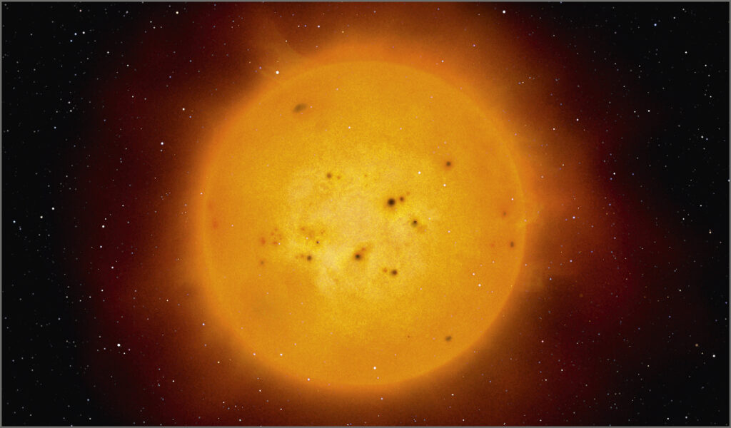
Rotating variables
Stars with light and dark regions show variation as the star rotates. The regions typically result from intense magnetic fields causing hot-spots or starspots on the surface of the star. Examples include:
Cor Caroli BY Draconis and SX Arietis
CM Tauri, the Crab Nebula pulsar, which is a rotating variable.
Spica, a non-eclipsing binary with elliptical components that change brightness depending on how they present to us.
AU Arietis, a close binary where the hot component’s radiation reflects off a cooler companion.
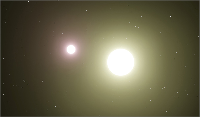
Close binary eclipsing systems
These star systems appear to change brightness because the component stars eclipse one another as seen from Earth. Among the many examples are:
Algol Beta Lyrae
RS Canum Venaticorum and Lambda Tauri
Some, like V0376 Pegasi vary in brightness due to orbiting exoplanets. Unequal components produce a deep primary eclipse and a shallow secondary eclipse.
EW Ursae Majoris-type variables have comparable ellipsoidal components producing similar primary and secondary eclipses.
Learning from irregularities
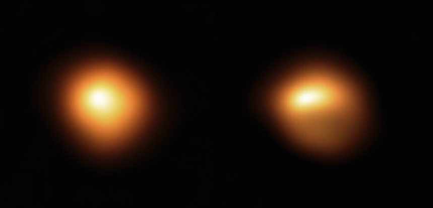
The light curves of irregular variable stars are extremely useful too. A long-period variable such as Betelgeuse (Alpha (α) Orionis) exhibits several periodic variations in brightness over different time spans and only by recording these over an extended period can the cycles be determined. In 2019 and into 2020 Betelgeuse became headline news as it unexpectedly faded. Known to be an old star close to the end of its life, this prompted many speculative predictions that the star was about to go supernova. It didn’t and the variation in brightness was subsequently found to be due to cooler dust blocking the star’s light. However, regular magnitude observations were in great demand over the fade period.
Cepheid variables, on the other hand, have light curves which show very regular periods. A groundbreaking discovery by Henrietta Swan Leavitt in 1908 showed the period to be directly linked to the star’s luminosity. Basically, by determining the period of a Cepheid, you can determine how luminous it should appear. It’s then possible to deduce how distant the star is in order to appear as bright as it does to us here on Earth. For this reason Cepheids became known as ‘standard candles’, and identified as an extremely important type of variable.
Although Betelgeuse is easy to see and a good starter, it also highlights a problem with red stars. Before we get to the reason why, let’s take a look at some guidelines to follow to help you become an accurate and prolific variable star observer.
Before making any observation, let your eyes experience at least 20 minutes of complete darkness, subsequently avoiding any form of artificial light until the observation has concluded. The only exception would be dim red light for illuminating your log book in order to record your observations. Avoid using a computer or phone to record observations, as even a red screen’s light plays havoc with dark adaptation.
We’ve already stated you shouldn’t research details of a variable’s state before making an observation. Doing so introduces bias which is bad science. Make the observation with a clear mind, recording whatever you see no matter how odd it may seem.
The issue with Betelgeuse applies to any star with a reddish tint, a common trait of intrinsic variables. The problem is that different eyes have different red-light sensitivities. Compare magnitude estimates of a red-hued variable to other results and you may find discrepancies. However, light curve shape should remain the same, along with total magnitude variation. Red stars also appear to brighten when viewed directly. This is awkward and the advice is to not stare at them for extended periods, instead developing a short glancing technique.
Other factors affecting variable star observations are sky quality, altitude above the horizon, and where the star and its comparisons sit in your field of view. Aim to move variables and comparison stars near the centre of the field of view when observing them.
Averted vision alert
When a variable is on the limit of visibility, it’s natural to use averted vision to try and squeeze as much sensitivity out of your eyes as possible. This requires you to look to the side of the dim target so its light falls on a more sensitive part of your retina. When you become accustomed to looking at fainter objects through the eyepiece of a telescope, averted vision becomes second nature and you may not be aware you’re even using it. However, for variable star observing, it’s imperative to note when averted vision has been used. Averted vision may attribute a brighter magnitude to the star than it deserves, potentially skewing the result.
Once you’re in the rhythm of observing variables regularly, you’ll find the process quick and efficient. Start with a handful of easy targets, expanding the list as your experience grows. Submit your results to a recognised association such as the BAA (British Astronomical Association, britastro.org), where they will be put to good use.
The fractional method
Use this technique to estimate a variable star’s brightness if you’re just starting out
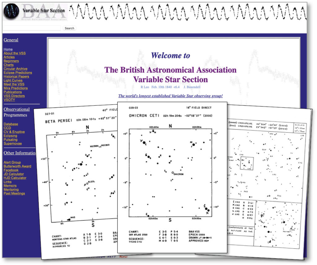
Choose a variable star and find a reference chart for it via the BAA (British Astronomical Association, britastro.org) or AAVSO (American Association of Variable Star Observers, aavso.org). Both organisations have charts for variable stars which identify non-varying comparison stars to use when estimating the variable’s brightness. Pick two stars, one brighter (A) and one dimmer (B) than the variable (V). If the difference in brightness between A and V equals that between V and B,
V is mid-way between A and B, and you’d write that as ‘A(1) V(1)B’; the brighter comparison is always presented first. If the difference between A and V were three times larger than that between V and B this would be written as ‘A(3)V(1) B’ and so on. You’re mentally dividing the difference in brightness between A and B into a number of parts, in this example 4, and placing the variable along that scale. If A’s magnitude was +3.7 and the real difference between A and B was 0.4 magnitudes, each ‘A(3)V(1) B’ division represents 0.4 ÷ 4, or 0.1 magnitudes. In this example, V is 0.1 magnitudes brighter than B and 0.3 magnitudes dimmer than A, making it mag. +3.7 – 0.3, or +3.4. The magnitude difference between A and B should be less than 0.6.
Six variable stars to get you started
These well-known variable stars are great to develop your observing skills on; their charts below have comparison stars’ magnitudes labelled
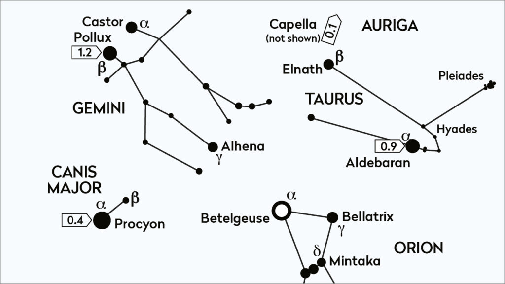
Betelgeuse (Alpha (α) Orionis)
Recommended equipment: Naked eye
An easy to find, long-period variable, sometimes tricky to estimate. It has semi-regular variation, typically mag. 0.0 to +1.6
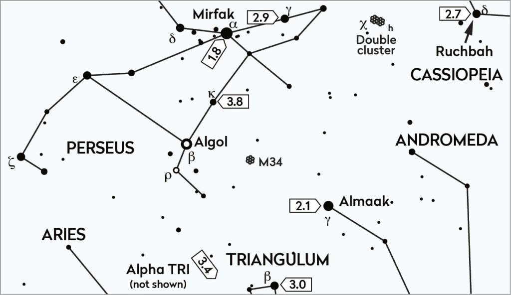
Algol (Beta (β) Persei)
Recommended equipment: Naked eye
An eclipsing binary system, which varies between mag. +2.1 to +3.4, with a period of 2.86 days.
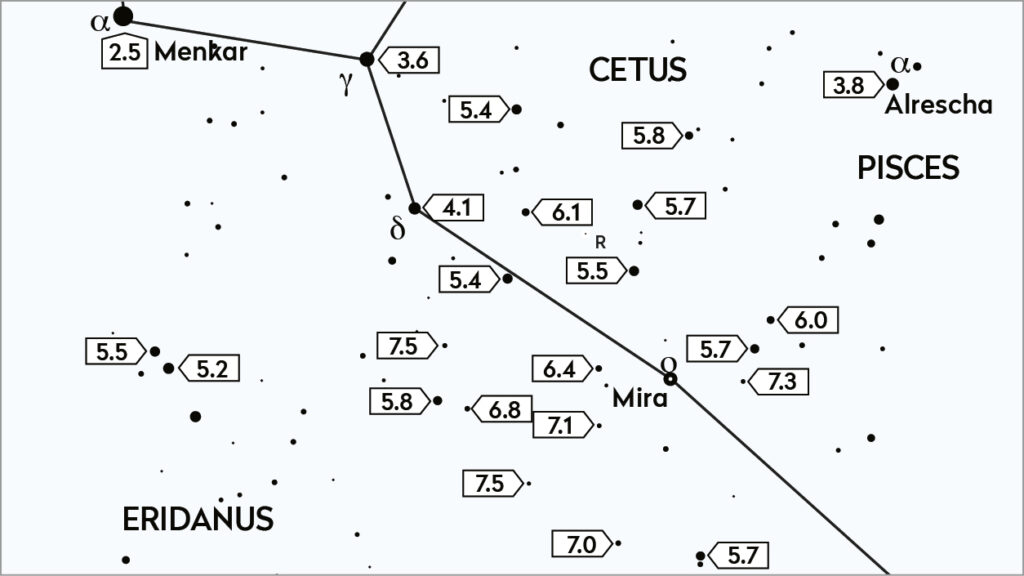
Mira (Omicron (ο) Ceti)
Recommended equipment: Naked eye, binoculars or small/medium telescope
The prototype of Mira-type pulsating variables. The magnitude range is +2.0 to +10.1 but can deviate, with a period of 332 days
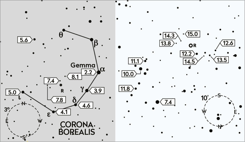
R-Coronae Borealis (R CrB)
Recommended equipment: Naked eye, binoculars or large telescope
An irregular eruptive variable, with a typical magnitude of +5.7 to +14.8. Its light curve can be very unpredictable
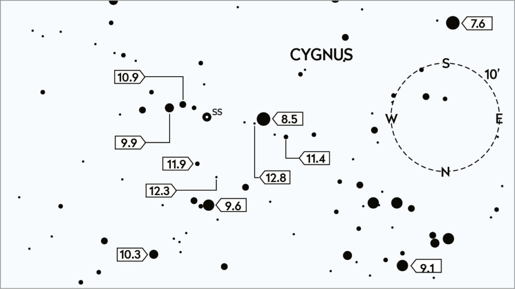
SS-Cygni
Recommended equipment: Small/medium telescope
A dwarf nova, with a magnitude of +7.7 to +12, it typically peaks for 1-2 days every 7-8 weeks.
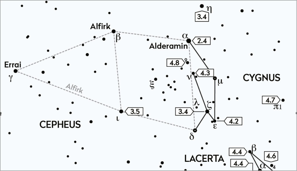
Delta (δ) Cephei
Recommended equipment: Naked eye
With a magnitude of +3.5 to +4.4 and a period of 5.3662 days, its rise to maximum brightness is faster than the following decline.
The Pogson step method
A technique to use when you are confident in estimating small changes in brightness
With experience, you should be able to visually estimate magnitude differences as small as 0.1. When you’re confident you can do this, consider using the Pogson step method.
Here, you choose a comparison star close in brightness to the variable (V) and estimate how many tenths of a magnitude it is brighter or dimmer. If you saw comparison star D was 0.2 magnitudes dimmer than V, you’d write this as ‘D-2’. It’s regarded as good practice to use more than one comparison to help smooth results and eliminate errors. For example, if you saw star C being 0.3 magnitudes brighter than V, write it as ‘C+3’.
After your observation you can use the magnitude table on your chart of the variable to determine the magnitudes of C and D, and then work out the two values for V. If they don’t quite match, average and round off if necessary. For example, if C is mag. +5.8, and D is mag. +6.2, this gives V amagnitude of +5.8 + 0.3, or mag. +6.1 from comparison star C; and +6.2 – 0.2, or mag. +6.0 from comparison star D. Take the average (+6.1 + +6.0) ÷ 2, to get +6.05, and round it off to get +6.1. If the variable can’t be seen, identify the faintest comparison star, for example F, and write the observation as ‘<F’.

Pete Lawrence is a skilled astro imager and a presenter on The Sky at Night.